![\includegraphics[width=8cm]{msgapphys}](img2336.png)
|
A symmetrical microstrip gap can be modeled by two open ends with a capacitive series coupling between the two ends. The physical layout is shown in fig. 11.6.
The equivalent ![]() -network of a microstrip gap is shown in figure
11.7. The values of the components are according to
[37] and [30].
-network of a microstrip gap is shown in figure
11.7. The values of the components are according to
[37] and [30].
![$\displaystyle C_S \textrm{ [pF] } = 500\cdot h\cdot\exp\left( -1.86\cdot\dfrac{...
... -0.785\cdot\sqrt{\dfrac{h}{W_1}}\cdot \dfrac{W_2}{W_1} \right) \right) \right)$](img2337.png) |
(11.193) |
 |
(11.194) | |
 |
(11.195) |
with
 |
(11.196) | |
 |
(11.197) | |
 |
(11.198) | |
 |
(11.199) | |
 |
(11.200) |
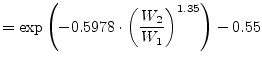
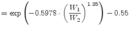
with ![]() and
and ![]() being the open end capacitances of a microstrip
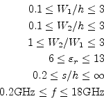
line (see eq. (11.192)). The numerical error of the
capacitive admittances is less than
being the open end capacitances of a microstrip
line (see eq. (11.192)). The numerical error of the
capacitive admittances is less than ![]() mS for
mS for
 |
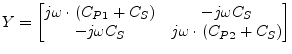
The Y-parameters for the given equivalent small signal circuit can be written as stated in eq. (11.201) and are easy to convert to scattering parameters.
![\includegraphics[width=12cm]{msgap}](img2349.png)